Sound Source Separation
Consider that you are a musician. So now, you already are a great enthusiast of signals — sound signals. Now suppose you are given an audio file to process. You play the audio and you find it very chaotic. It has a combination of instruments playing all together. But given that you are a musician — an adventurous one — you decide to experiment with the audio file. You decide to remove a few instruments or maybe combine only for certain segments. The problem is that there are no individual recordings of the instruments and producing those might require a lot of time. So how do you do separate the audio from each instrument? This situation is analogous to signal source separation problem.
Source separation, blind signal separation (BSS) or blind source separation, is the separation of a set of source signals from a set of mixed signals, without the aid of information (or with very little information) about the source signals or the mixing process.
It is most commonly applied in digital signal processing and involves the analysis of mixtures of signals; the objective is to recover the original component signals from a mixture signal.

The classical example of a source separation problem is the cocktail party problem, where a number of people are talking simultaneously in a room (for example, at a cocktail party), and a listener is trying to follow one of the discussions. The human brain can handle this sort of auditory source separation problem, but it is a difficult problem in digital signal processing.
It can be very well established that “All signals are sum of sines”. And thus, if you can construct a signal using sines, you can deconstruct signals into its constituent sines. Once the original signal is deconstructed, you can see and analyze the different constituent signals. Consider these examples –
1) If you deconstruct radio waves, you can choose which particular frequency–or station–you want to listen to.
2) If you deconstruct audio waves into different frequencies such as bass and treble, you can alter the tones or frequencies to boost certain sounds to remove unwanted noise.
3) If you deconstruct earthquake vibrations of varying speeds and strengths, you can optimize building designs to avoid the strongest vibrations.
4) If you deconstruct computer data, you can ignore the least important frequencies and lead to more compact representations in memory, otherwise known as file compression.
Example
Now, that we have established the definition of signal source separation and the reason why it is necessary; let’s dig deeper into sound signals and source separation in case of sounds by experimenting with some code. Let us assume the formal problem statement as follows.
Analog/Digital acoustic data is available in time domain. The acoustic data is a mix of multiple acoustic sources. The issue at hand is to segregate and clip out data of specific acoustic sources. The segregated clipped out data to be made available in form of audio files for end user. Fundamental frequencies of various acoustic sources are known.
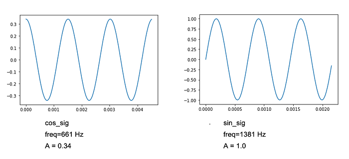
To visualize and solve this problem lets create some dummy sine audio signals. Let’s say the fundamental frequency of first wave is 661 Hz and other wave is 1381 Hz with a phase difference of 90 (one is Cos, the other is Sine). We are using amplitudes to be 0.34 and 1.0 respectively, but they can be any. To do so, we use the library ThinkDSP which makes this task super easy
from thinkdsp import CosSignal, SinSignal # Signal Source 1
cos_sig = CosSignal(freq=661, amp=0.34, offset=0)# Signal Source 2
sin_sig = SinSignal(freq=1381, amp=1.0, offset=0)
The visualization of the cos and sine signal is as follows. They look very similar, although note the X scale to understand that the cycles in higher frequency wave at 1381 Hz are closer than the cycles in 661 Hz wave.
# Visualizing Cos Signal
cos_sig.plot(framerate=44100)# Visualizing Sin Signal
sin_sig.plot(framerate = 44100)

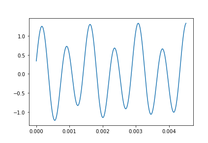
Let us combine these two waves and call it mix. The visualization is the resultant wave of the two waves, where the maximum of both the waves is seen at any particular time.
# Combine source signals
mix = cos_sig + sin_sig

# Visualizing combined Mix signal
mix.plot(framerate = 44100)
Now for a more believable observation, lets listen to the audio waves generated.
We can clearly notice that the mix is the combination of the constituent sine audios.
If we observe the spectrum graph of the mix signal, we clearly see that the only frequencies present are at 661 and 1381, and the height of the bars correspondents with the amplitude set.
# Spectrum graph for mixed signal
(mix_audio.make_spectrum()).plot()
Now that we have our audio signals, lets save them for further use.
# Saving the encodings as files for later usemix_audio.write('mix_audio.wav')
sin_audio.write('sin_audio.wav')
cos_audio.write('cos_audio.wav')
Attempting Separation
We will apply the following steps to attempt separation of the mixed signal:
- Convert the signal from time domain to frequency domain using FFT
- Filter the signal by known fundamental frequencies.
- Convert the filtered signal from frequency domain to time domain using IFFT
You can find the entire code here.
For this, we read the mix audio file using wavfile.read() from scipy.io package. This function returns the sampling frequency fs and an array of discrete time samples mix_data as follows
from scipy.io import wavfile
# Read the audio file
fs, mix_data = wavfile.read('mix_audio.wav')
We define the fundamental frequencies f0_1 = 661 and f0_2= 1381 from the first half of this post, and apply Fast Fourier Transform on the mix_data to get the frequency domain signal.
from scipy.fftpack import fft, ifft
import numpy as np

# Known Fundamental Frequencies
f0_1 = 661
f0_2 = 1381

# Applying FFT
fft_data = np.fft.fft(mix_data)
The frequency domain data when plotted gives the frequency spectrum as we had seen before.
import matplotlib.pyplot as plt# Plotting the FFT magnitude (spectrum graph)
plt.plot(np.abs(fft_data))

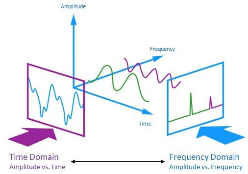
To quickly understand how FFT and audio signal is related; check the following image.

As seen above, an audio signal is a set of curves in the (amplitude, time, frequency) space. And by performing an FFT we essentially change the perspective of looking at the audio signal.
Now, coming to the main functions filter_freq(lower, higher, fft_data) and get_audio(fft_data).
def filter_freq(lower, higher, fft_data):
    '''
    This function acts as band pass filter and returns the fft_data
    with frequencies in the range from lower to higher (both
    inclusive).
    '''
    filtered = fft_data.copy()
    for i in range(len(filtered)//2):
        if i<lower or i>higher:
            filtered[i]  = 0            # make f(k)   component zero
            filtered[-i] = 0            # make f(n-k) component zero
    return filtered
The filter_freq function zeroes out all the frequency data other than the range lower to higher. The important thing to notice in this function is that FFT is symmetric / mirrored [3], and thus we need to zero out the mirrored component as well during filtering. Hence, we do F(k) = F(N-k) = 0 for all k values out of the range (lower, higher). The filter_freq in the end returns the filtered version of fft_data, thus retaining only the range of frequency required by the user and acts like a band pass filter.
def get_audio(fft_data):
    '''
    This function encodes the fft_data back into audio format.
    Applies IFFT.
    '''
    return np.real(np.fft.ifft(fft_data)).astype(np.int16)
The get_audio() function takes fft_data as input and converts it to real discrete time samples by using IFFT. The returned array when decoded at the original sampling frequency should play filtered signal.
Now using these functions let’s play the signals filtered at their fundamental frequency.
import IPython.display as ipd# 1. Filter Mixed Signal at Fundamental Frequency f0_1.
source_1_fft = filter_freq(f0_1, f0_1, fft_data)#2. Get Audio encoding.
audio_1 = get_audio(source_1_fft)#3. Play the Audio.
ipd.Audio(audio_1, rate=fs)
The 661 Hz filtered signal sounds as follows
The 1381 Hz filtered signal sounds as follows
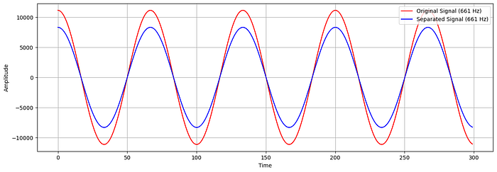
The results are great, they sound exactly like the originals. But are they exactly the same? Let’s explore. So, there is a difference in the extracted audio signals if we explore the array values. As the numerical values don’t make much sense, lets plot the data of a few samples from the original and the separated source signal.

Aloha! The two waves have the same frequency cycles, and differ only in amplitudes. What does that mean? It simply signifies that the separated signal will have different volume levels. Can we correct this? Yes, surely. We just have to scale the values. However, we didn’t do the scaling for the sake of simplicity and as the resultant sound effect produced will be the same and will slightly differ in terms of volume level, which can be adjusted anytime!
The Glitch in the Matrix (literally…)
Finally, we were able to solve this problem of sound source separation! Umm.. yes and no. The example that we solved was far too ideal compared to the real world. When it comes to real world sound signals. Each source will have a range of frequencies that it will operate in. Lets see how does a pluck on Guitar in real world sounds (though, even this is generated on a virtual guitar 😛).
The spectrogram of this sound effect is as follows.

But its still manageable. We can filter a range of frequencies. That’s not an issue. The real issue arises in case of overlaps. Different sound sources may have a common frequency range. And when such a frequency range occurs in the audio file, how do you decide that this segment belongs to which sound source. Maybe you decide by the known maximum amplitude of the sound sources or maybe you already have time mappings for sound sources or maybe you allow it to belong to all the sound sources present.
“The fundamental problem in sound separation is that when two or more sounds overlap with each other in time and frequency, separation is difficult and there is no general method to resolve the component sounds.”
By making some assumptions of the underlying signals, the parameters of the sources can be estimated from the mixture signals, and signals which are perceptually close to the original ones can be synthesized.
The Real-World Approaches
The FFT approach is simply naïve and cannot be applied to real world directly. It has to be tuned a lot and still has a lot of room for research. There are a few statistical approaches that in general detect the un-overlapped parts and then reconstruct the overlapped parts by various estimations and assumptions.[4] But these approaches are not very realistic as they require expert attention in the process. The sole purpose of exploring this problem is to make machine do the underlying task and give consumable result.
The more interesting solutions are employing deep learning techniques and making use of advances in the machine learning field. Spleeter is one such solution.[5] It is a library that can be used to train models with a set of isolated samples and mixed samples. It also comes with some pretrained models that give quite a performance. You can check their project on GitHub.[6] Just check out this interesting thread by Tweep “Andy Baio” on Spleeter.
References
[1] “Signal Separation”, Wikipedia, https://en.wikipedia.org/wiki/Signal_separation
[2] “Understanding FFTs and Windowing”, NI, http://download.ni.com/evaluation/pxi/Understanding%20FFTs%20and%2 0Windowing.pdf
[3] “Why is FFT mirrored?”, DSP StackExchange, https://dsp.stackexchange.com/questions/4825/why-is-the-fft-mirrored/4827#4827
[4] “Musical Sound Source Separation based on Computation Auditory Scene Analysis”, Jinyu Han, Interactive Audio Lab, Northwestern University, https://users.cs.northwestern.edu/~pardo/courses/eecs352/lectures/source%20separation.pdf
[5] “Spleeter by deezer”, https://deezer.io/releasing-spleeter-deezer-r-d-source-separation-engine-2b88985e797e
[6] “Spleeter — GitHub repository”, https://github.com/deezer/spleeter
[7] “Allen Downey — Introduction to Digital Signal Processing — Pycon 2017”, YouTube, https://www.youtube.com/watch?v=UOIllEyajGs&list=PLROS-L5Pj_CTfPoC60JKnFQZrC_m-9ZQb
[8] Experiment with filters on wav files, Stanford Edu, https://web.stanford.edu/class/archive/engr/engr40m.1178/slides/filter.py
